Composite Material Testing – The Challenges of Batch-to-Batch Variation and How to Manage Them
- 29th June 2018
- Elliot Fleet
- Reading time: about 13 minutes
Statistics is a branch of mathematics that deals with managing data and evaluating logically how well it fits a preconceived pattern or model. Similarly a large part of composites R&D and materials science is concerned with generating data and using it to support a hypothesis. The use of statistical methods is therefore absolutely critical to R&D in materials. Unfortunately, statistics is relatively poorly understood and constantly misrepresented in academia, industry and the media.
The aim of this article is not to go into detail or the theories of statistics itself; there are numerous resources available online that do just that. The aim is to highlight, with a relatable example, a common pitfall. It doesn’t require much in the way of background knowledge other than a basic working knowledge of the following:
x̅ – Sample mean (average): the sum of all the numbers in the set divided by the amount of numbers in the set. Excel formula: AVERAGE
s – Sample standard deviation: used as a measure of spread from the mean. Excel formula: STDEV.S
CV – Coefficient of variation (%): the standard deviation divided by the mean expressed as a percentage. This can be a more relatable value than the standard deviation. For most mechanical testing jobs, for example, 5 to 10% is fairly common.
CI95 – 95% Confidence Interval: based on Student’s t-intervals if you were to repeat the exact experiment 100 times, the true population average would be within the error bars approximately 95 times. Excel formula: CONFIDENCE.T(0.05,s,n). This is not quite the same as saying we are 95% confident that the population mean is between the error bars but this distinction is minor.
Student’s t-test: a method of testing hypotheses about the mean of a small sample drawn from a normally distributed population when the population standard deviation is unknown [1]. It is often used to compare a treated sample against a control or known value. The test produces a “p-value” which, if lower than a specified value, (typically 0.05) suggests that the treatment effect is significant. In statistical jargon “there is a 95% chance that the samples are drawn from different populations.”
A potential difficulty for the materials scientist is that the vast majority of text books and online articles are written predominantly for social scientists or medical researchers and often use examples involving survey data or massively complicated data sets. It can be difficult for engineers and scientists from other disciplines to see how the examples relate. However, the examples given are often more applicable than you might think at first glance. An important first step is to understand what writers mean by the phrase “the population”.
The population
The “population” is a word that gets used an awful lot in statistical texts. The most obvious valid example is to use the word at face value to mean the population of a country. In these cases the population is often large but it is still finite. A company that makes clothing might be interested to understand how factors like “height” might vary so that they can produce a range that fits 95% of the market. They might also want to make more units in certain sizes and fewer units in rarer sizes. It is not reasonable to go and measure every person in the country so the best approach is usually to measure a sample of people and make estimations based on this sample. The quality of the estimate will depend on ensuring that the sample is large enough and represents the wider population. For instance, a poor sample would be the measured heights of a group of people all living in a region with shared genetic propensity towards being very tall. The use of this sample would make your population estimate inaccurate even if there were a lot of measurements.
So what does “the population” mean in materials science?
In materials science we are often testing physical specimens or aliquots of material. We want to control some factors (keep them the same or similar) and change other factors or apply a treatment (to learn what the effect is on our material).
In this case the definition of population is more abstract. There are not a fixed number of specimens dispersed around the country awaiting collection; they usually have to be produced in some sort of process. The population, in materials science terms, could be described as every specimen that has and could ever be made under the specified conditions and can be considered effectively infinite. You are never going to measure the population only estimate it. If you make a new set you are not increasing the population.
Example
The following example uses model data generated using a random number generation service [2] to illustrate my point. Let us say we have an additive that we think might increase the lap shear strength of a one part adhesive. We devise a simple experiment in which we test the lap shear strength of the adhesive with and without the additive.
Here is our hypothetical process:
- We mix a small batch of adhesive with additive by hand
- We prepare the surface of our substrates (e.g. abrade and clean with solvent)
- We spread the adhesive on our substrates, clamp them together and cure them in an oven overnight (6 control, 6 with additive)
- The following day after, conditioning the specimens, we test the lap shear strength on a universal test machine.
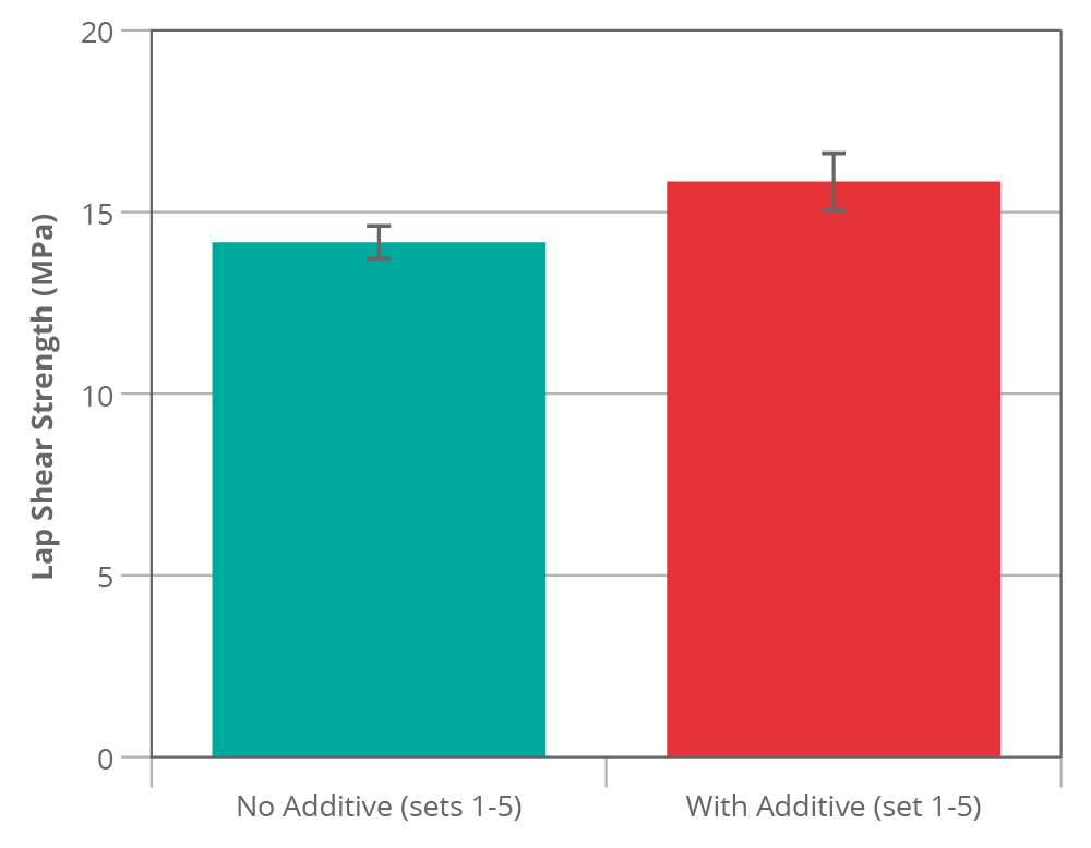
We then get the following results:
| Lap Shear Strength (MPa) | ||
|---|---|---|
| Specimen | No Additive | With Additive |
| 1 | 11.96 | 14.97 |
| 2 | 15.71 | 16.26 |
| 3 | 15.29 | 14.76 |
| 4 | 15.27 | 13.49 |
| 5 | 13.35 | 15.18 |
| 6 | 14.62 | 15.24 |
| x̄ | 14.37 | 14.98 |
| s | 1.44 | 0.90 |
| CV | 10% | 6% |
| CI95 | 1.51 | 0.94 |
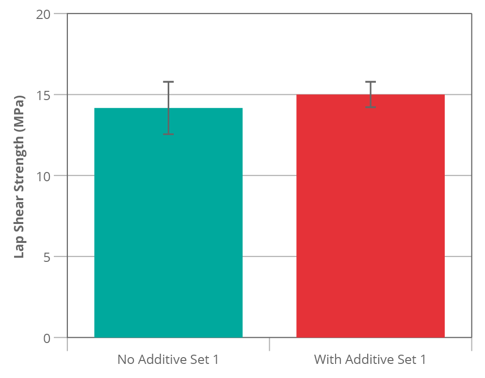
The results are fairly uninspiring right? There might be a slight increase in strength as a result of putting the additive in but it is minor. The error bars (95% confidence interval) also overlap a lot which suggests if we were to apply a formal statistical test to the data (such as a t-test) we are unlikely to conclude that there is a difference [3].
We could stop at his point and reject the effectiveness of the additive but would this be correct?
Let us consider what the populations might be. We are controlling for differences in the adhesive batch or age because we produced the samples from the same batch at the same time. We tried to control for the influence of the oven by curing both sets together. The “no additive” group is a sample from a population consisting of all possible samples made with this exact adhesive specification and prepared in the way described under the same conditions. Each specimen is prepared (glued) separately by hand which might lead to a high variation due to differences in bond thickness (for example). Despite the variation and the relatively low number of specimens the control sample is a reasonable approximation of its population.
What happens if we make four new control sets from the same batch of adhesive?
| Lap Shear Strength without additive (MPa) | |||||
|---|---|---|---|---|---|
| Specimen | 1st Set (as above) | 2nd Set | 3rd Set | 4th Set | 5th Set |
| 1 | 11.96 | 14.41 | 14.66 | 13.12 | 15.53 |
| 2 | 15.71 | 16.77 | 14.46 | 14.69 | 13.45 |
| 3 | 15.29 | 14.87 | 13.31 | 14.70 | 14.32 |
| 4 | 15.27 | 13.76 | 13.58 | 13.33 | 15.05 |
| 5 | 13.35 | 14.91 | 13.78 | 14.55 | 14.32 |
| 6 | 14.62 | 12.97 | 14.04 | 14.82 | 15.46 |
| x̅ | 14.37 | 14.62 | 13.97 | 14.20 | 14.69 |
| s | 1.44 | 1.29 | 0.52 | 0.76 | 0.80 |
| CV | 10% | 9% | 4% | 5% | 5% |
| CI95 | 1.51 | 1.35 | 0.54 | 0.80 | 0.84 |
| Combined x̅ | 14.37 | ||||
| Combined s | 0.99 | ||||
| Combined CV | 6.9% | ||||
| Combined CI95 | 0.37 | ||||
The combined mean of all the test sets together is 14.37 MPa (it is complete co-incidence that this is the same as the first average). We do, however, know the average more precisely now (± 0.37 MPa). The sample standard deviation differs a fair bit between groups but this is a normal occurrence in small sample sizes.
Now let’s consider the case of the additive. In the first set of results the variation (and therefore the error bars) was actually narrower than the unfilled group. It would be tempting to assume that the results are reliable but does the sample properly represent the population filled adhesive samples? To find out we make up four new additive mixes and test these as before.
| Lap Shear Strength with additive (MPa) | |||||
|---|---|---|---|---|---|
| Specimen | 1st Set (as above) | 2nd Set | 3rd Set | 4th Set | 5th Set |
| 1 | 14.97 | 15.45 | 17.53 | 15.24 | 20.51 |
| 2 | 16.26 | 16.53 | 18.28 | 17.37 | 21.86 |
| 3 | 14.76 | 15.71 | 19.79 | 15.79 | 20.29 |
| 4 | 13.49 | 15.46 | 17.69 | 15.55 | 18.18 |
| 5 | 15.18 | 18.85 | 18.92 | 14.17 | 19.21 |
| 6 | 15.24 | 15.70 | 19.72 | 15.76 | 20.13 |
| x̅ | 14.98 | 16.28 | 18.66 | 15.65 | 20.03 |
| s | 0.90 | 1.32 | 0.98 | 1.04 | 1.25 |
| CV | 6% | 8% | 5% | 7% | 6% |
| CI95 | 0.94 | 1.38 | 1.03 | 1.09 | 1.31 |
| Combined x̅ | 17.12 | ||||
| Combined s | 2.20 | ||||
| Combined CV | 12.8% | ||||
| Combined CI95 | 0.82 | ||||
After performing the new experiments a different picture starts to emerge, while the individual groups show a similar (reasonable) level of variation compared to the control there is a lot of difference between the groups that we did not see in the control. Some other factor is causing an increase in variation.
One likely explanation for this is the additive mixing step. Are we introducing scatter in our results by failing to properly control our mixing? Perhaps some batches were better mixed than others? In this case our first set might not be a good representation of the population as this set of specimens was made from a batch of adhesive that was poorly mixed. This concept can be applied to almost anything that is grouped into batches. FRP composite laminates prepared by hand layup are particularly susceptible to variation due to fibre alignment and consolidation differences.
What would have happened if by chance we had first measured set 3?
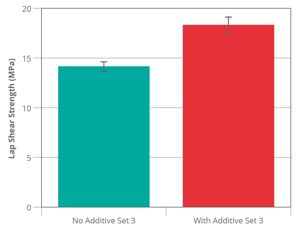
I think many people would have looked at that data and assume the additive is making a big difference ~34% improvement. Based on this result we could be tempted to drop other avenues of research and focus on optimising this system since it looks so promising. A t-test on this data would probably indicate that there is a high chance that these populations are different (i.e. the additive is working) [4].
Just to be clear, the data for figure 1 and figure 2 was generated from the same populations and both had an equal chance of occurring yet they seem to indicate conflicting conclusions. The error bars (and t-test) derived from the variation within-batch do not represent the full picture, all they tell us is that a particular mixed adhesive batch performed better than the control. If a process variation is not understood then a particular batch can perform better or worse by random chance just as a single test specimen in a sample can perform better or worse.
If we look at all five groups we can see that if we had taken each set on its own any conclusion we try to draw could be different each time (figure 3). Set 1 shows no real difference, sets 2 and 4 show a borderline improvement and sets 3 and 5 show quite a big improvement.
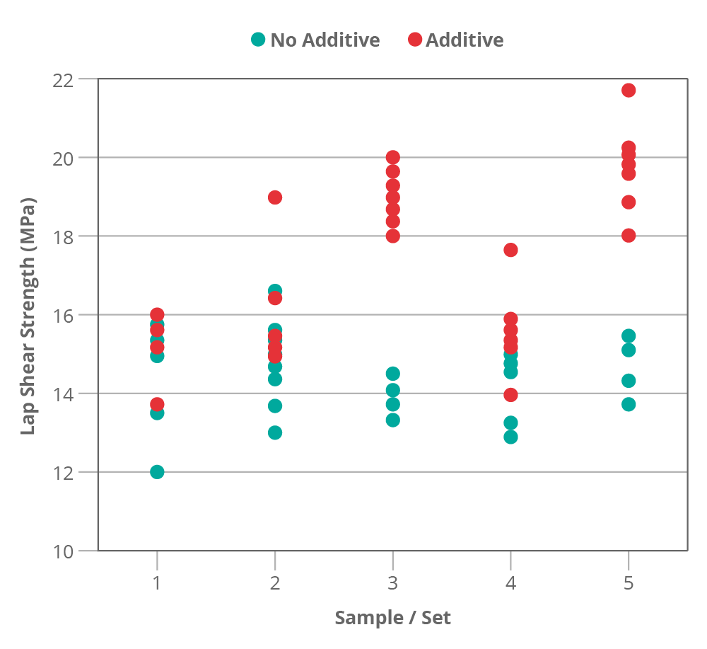
The real story is, of course, somewhere in between. The new combined mean of 17.12 MPa is a much better representation of the population. The treated group appears to be significantly [5] higher than the control (~19% better). This is a reasonable result for our additive.
What do we learn from this?
The first thing that we learn is that we may need to look into our mixing process; can it be more controlled or automated? Sometimes improvements can be made but also sometimes improvements are not practical.
Be very careful when doing tests that rely on specimens that come from a common grouping, e.g. batch, test plaque or treatment process. A grouping can introduce the possibility of biasing the results. If you rely on standard deviation or confidence intervals derived from a single set derived from a grouping you can get a false idea of accuracy.
In composite materials R&D these groupings are everywhere; nominally identical composite specimens produced from prepreg for example can be members of various different groups:
- Fibre batch
- Textile (weaver) batch
- Resin batch
- Prepreg batch
- Prepreg outlife (date)
- Cure run (e.g. same oven/autoclave)
- Individual laminate (possibly with variation from hand-layup or specimen alignment)
- Ambient conditions
It can be expensive and time consuming to produce enough test specimens from sufficiently different groups; often we are not in a position to produce as many as we would like. Nevertheless, as a minimum it is good practice to include more than one set of specimens. The materials qualification process for aerospace, for example, requires specific minimum numbers of raw material batches. If you are forced to stick to one set then please be open minded to the very high risk of being misled. Sometimes the cost savings provided by reducing the number of experiments can be completely overshadowed by the cost of subsequently following the wrong tangent! It is also perfectly possible to encounter an apparently significant result when there is really no difference in the populations.
For FRP composites the experimental error derived from specimens machined from a single laminate or plate nearly always appears lower than the same number of specimens from different plates and (in comparison to the “height” measurements) may just happen to be a sample from a “Tall” region.
One other thing…
Unlike real life data, the model data presented was generated so I actually know what the population values were (but it is the sort of thing I have encountered in the wild).
The control adhesive was 14.0 MPa with a population standard deviation of 1.2 MPa and no batch-to-batch variation.
- The additive adhesive was 16.8 MPa (exactly 20% higher) with 1.2 MPa within-batch standard deviation and 1.0 MPa between-batch standard deviation.
I could have set the within-batch variation to be much lower than the between-batch variation which would have exaggerated the effect but I thought this might look unrealistic for this type of test.
[1] It can be performed using the excel “analysis toolbox” or using free online tools from providers such as Graphpad.
[2] Haahr, M. (2018, June 7). RANDOM.ORG: True Random Number Service. Retrieved from https://www.random.org (Gaussian Random Number Generator).
[3] This assumption is correct; the P value is equal to 0.39 with 10 degrees of freedom which is significantly higher than the 0.05 level. Based on this we would not reject the idea that the samples came from identical populations.
[4] A t-test shows exactly that, a p value is calculated to be less than 0.0001 with 10 degrees of freedom which is considered extremely statistically significant.
[5] According to a t-test it is extremely statistically significant p<0.0001 at 58 degrees of freedom.
Found this article useful? We have a full range of services to help you...

Materials Characterisation & Testing
We have an extensive suite of testing facilities for characterising polymers and composites, coupled with the necessary expertise to interpret and advise upon test results.
Testing composites...About the author


News